The William H. Hannon Library hosts over 40 programs every year. Like many colleges and universities, Loyola Marymount University has multiple public calendars, bulletin boards and online spaces where students, faculty and staff go to find information about upcoming events. To rise above the surfeit of campus programming options for our users, it's important to make sure each space is populated with library programming information in a timely fashion.

With so many events happening throughout the year and a minimum of 14 routine channels for programming outreach (e.g. university calendar, faculty intranet, Facebook event, library homepage, print flier, email invite, etc.), I have found that setting artificial deadlines for sending information out via each channel is the easiest way for me to stay on track and to space out the communications work needed to push out as much content as possible. To that end, conditional formatting in Microsoft Excel and Google Spreadsheets is an indispensable tool.
What is conditional formatting?
Conditional formatting in Excel allows you to create rules that change the way a cell appears (e.g., its color) based on specific parameters. For example, if a cell's content contains a number that falls within a specific range, or if you want to visualize the degree to which one cell's content relates to other cells in the same column/row, you can use conditional formatting to give the cell a specific color, border or font. This can help you quickly identify meaningful information in the spreadsheet. Most importantly, conditional formatting is dynamic: it automatically updates if the cell's content changes based on other factors or formulas.
How can I use conditional formatting in library programming outreach?
In order to track important deadlines for distributing content about library programs, I've set up an array of conditionally formatted spreadsheets to let me know when and how I should prioritize specific content. For example, I typically try to have library events posted to the university's main calendar four to six months out. I try to make sure the event is mentioned at specific intervals on our social media channels in the month leading up to the event (as well as after). Additionally, I often create large print posters for on campus a-frames, banners for the library homepage, and graphics for digital screens that are installed across campus. Ideally, these print and digital materials are pushed out one or two months before the event.
Of course, I don't utilize every communication channel available to me for every library program, but even assuming I use half of the channels for every event we plan this year, that means there are over 300 opportunities for telling our students, faculty and staff about library programs. To ensure that I hit as many of these as possible, I use conditional formatting to help me keep track of what is coming next.
What follows is a step-by-step process for setting this up in Excel.
Part 1: Set up your deadlines in Excel
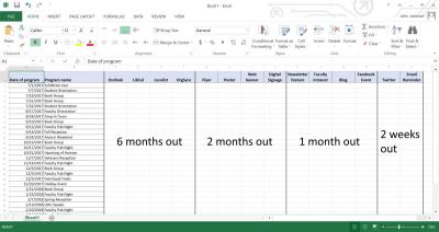
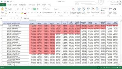
1. Open a new Excel sheet. In column A starting on row 2, list the dates for each of your library programs.
2. For the sake of simplicity, list the corresponding event titles in column B. You can add adjacent columns for the project leads, event locations, etc.
3. Next, we'll create our headers. In row 1 of columns C-P (or wherever your columns end), list each of the outreach/communication platforms to which you typically push content about your event. These should be arranged in columns left to right from first action to the last action, leading up to the date of the event. For example, in my spreadsheet, I have Outlook, Libcal, Localist and OrgSync in columns C-F because those are the first and earliest places where I want to post programming information. Moving to the right in columns G-J, I have items I want completed two months out, and so on.
4. Next we will tell Excel to interpret these columns as dates. To do so, highlight all the columns C-P and right click. Select "Format Cells." Select "Date" in the Categories column.
5. In column C, select the cell in the row that corresponds to the first date (e.g. C2). Type in the following formula: "=[Cell that contains program date]-[number of days before event]." So if my row is six months out, I would input "=A2-180". Hit enter to input the formula.
6. The cell should now automatically show a date that is exactly 180 days prior to the date in column A of the corresponding row.
7. Now that you have entered the date calculation in one cell, we will update the rest of the cells in that column. Select the cell in column C that you just edited (e.g. C2). A small green box should appear in the bottom right corner of the cell. Click and drag that box to the bottom of your column to copy the formula in each cell. This should populate all the cells in column C with dates 180 days prior to the corresponding dates in column A.
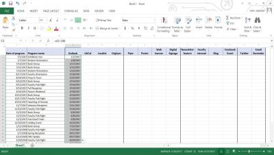
8. Repeat steps 5-7 for each column and change the number of days before the event accordingly, e.g. "=A2-60" for two months out, "=A2-14" for two weeks out, etc.
Part 2: Conditionally formatting the cells
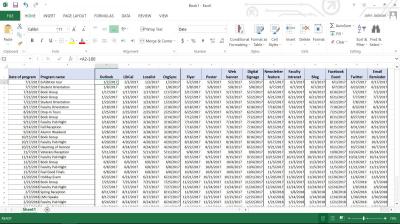
1. Select all the cells that contain dates in columns C-P.
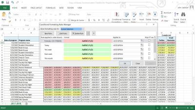
2. Select "Conditional Formatting > Manage Rules" from the ribbon.
3. Select "New Rule."
4. Select "Use a formula to determine which cells to format."
5. In the entry box, enter this formula: "=C2<TODAY()" (where C2 is the top left cell in your table of dates).
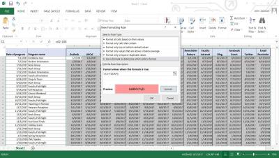
6. Select the formatting you desire. I used a light red color since this will indicate any cells that contain deadlines that have passed.
7. Click OK. This will cause cells with any dates in the past to turn red.
8. We now need to create conditional rules for dates that are in the future. This is much simpler. From the ribbon, select "Conditional Formatting > Highlight Cells Rules > A Date Occurring..."
9. Set up highlighting rules for Today, This Week, Next Week, This Month and Next Month. (I have Today, This Week and Next Week as green; This Month and Next Month are yellow). It's important to keep the rules in this order, listed top to bottom in the "Rule (applied in order shown)" column of the Conditional Formatting Rules Manager. Make sure the cell range includes all the cells in your table. You can always review and edit this in the Rules Manager.
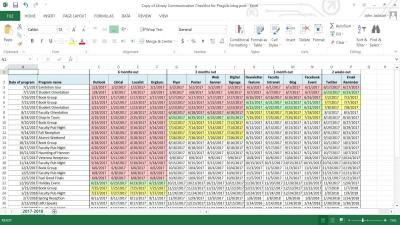
The final product (see below) will highlight any cells with past dates as red, any cells with dates between today and the end of next week as green, and any date between the end of next week and the end of next month as yellow. At a glance, I can now see exactly which communication channels I need to be using, for what purpose and when.
You can also set up conditional formatting in Google Spreadsheets using a process similar to the step-by-step one outlined above. Use conditional formatting to set artificial deadlines based on a target execution date for planning social media campaigns, creating exhibition installation workflows, planning out academic search committee work, and more!